Overview Link to heading

In this article I discuss my experience modeling data pipelines with the R package {targets} (Landau 2023) and some of the principles I follow in constructing them.

{targets} pipelines are a significant departure from the monolithic linear data workflows that are common in data science and which I myself have used heavily in the past (you can still see one at work in the ICJ corpus). Declarative workflows break up the pipeline into different components that are run in an order determined by the {targets} framework and the interlinked dependencies of the individual components.

This has many benefits. In particular, this type of pipeline significantly decreases development time, is easier to fix when broken and allows for shorter development increments. It is possible to spend an hour here and there instead of having to reserve an entire afternoon while working through a linear pipeline.

The downside is a fair amount of additional work when setting up the pipeline and the added intellectual complexity of the {targets} framework, but on the whole I am very satisfied will never go back to linear workflows (except for minor analyses).

I won’t claim that the principles for modeling pipelines presented in this article are best practice or comprehensive, but there are nevertheless some finer points that colleagues may appreciate.

Data Workflow Link to heading

If you follow my work you may have seen me post striking neon-on-black network visualizations of my data pipelines. I use these for three purposes:

1. Check the structure of my computations
2. Discuss the details of my work with a technical audience
3. Explain the general outline of data workflows to a non-technical audience

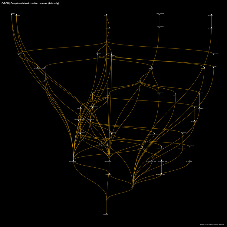
The most common visual I use to display pipelines is a network representation of the data workflow, also called a directed acyclic graph (DAG). Data workflow means that the diagram below includes only targets, the primary data components of the pipeline. Excluded are functions (i.e. computational instructions) and global variables.

Each target is a self-contained part of the pipeline that is computed in its own R process, with a specified reproducible seed and with its output stored as an individual R object, which can be accessed individually with tar_load() or tar_read(). Every target is defined by three elements:

1. Data input
2. Code
3. Data output

The small white dots in this diagram show the output and the link to the input(s), but not the functions. Target outputs usually are vectors or data frames (in my case almost always data.tables). Sometimes these vectors reference files on disk (e.g. when a target downloads thousands of PDF files). The framework computes hashes of all stored results (including references files on disk) and tracks changes to them. When the pipeline runs it automatically skips over targets that have already been computed and for which input and output remain unchanged. This feature alone makes it worthwhile to build {targets} pipelines.

I almost always use a targets-only visual of the workflow. Why?

1. The full structure (including functions) and globals becomes cluttered very quickly even with moderately-sized pipelines
2. A data pipeline is about the flow of the data, everything else is incidental to it
3. I find it easier to anchor my inspection of the code with data targets and then look at the associated function in the pipeline manifest .Rmd if there is an issue
4. It is visually more attractive

When I review the pipeline diagram, I always ask myself the same questions:

1. Are there dangling targets?
2. Are all targets connected to the proper upstream/downstream targets?
3. Does the overall pipeline concept make sense?

Dangling targets tend to happen fairly often during development, particularly when I’ve written all the necessary functional code but have forgotten to add downstream targets to the pipeline. Visual inspection shows this quickly. Sometimes I also comment out parts of the pipeline because I am working on upstream parts where frequent changes would cause the downstream part to rerun often. Visual inspection reminds me to uncomment these parts when I am done with upstream development work.

Checking proper connections is more tricky, but there are some elements of my own modeling style that are prone to improper links, so I re-check them often. For example, I tend to build a preliminary metadata download manifest from whatever database or file set I am currently extracting data from, but this often requires additional cleaning before I run the full data content extraction. Sometimes I continue to work on the pipeline before I have done the cleaning, so I hook up the preliminary data to downstream targets. When I add the cleaned download manifest to the pipeline I always check if I’ve severed the downstream connections with the preliminary data and added the final download manifest as a data source.

Most importantly, the overall workflow needs to make sense. If the pipeline structure is all over the place and doesn’t seem very intelligible I try to redesign the pipeline to make the process clearer, group similar targets together in the manifest and workflow and so on. Mistakes in programming happen more frequently if structure is poor, one of the reasons why re-use of functions and use of control flow is encouraged instead of burying problems under mountains of code.

Modeling Targets Link to heading

The construction of individual targets is more of an art than a science. At its core, each target can be thought of as a building block or component of the full workflow. The {targets} package forces you to use a single R expression (commonly a custom function) to create each target.¹

The question is then, how much should you fit into each target and its associated function? There are several criteria I use to decide:

• What is the runtime of the target?
• Can I avoid re-running computations by creating new targets?
• How often will I be refactoring/fixing the target?
• How interested am I in the results for a specific step of the workflow?
• Can I collect several related computations into a conceptual unit?
• Does it improve intelligibility in the context of the entire pipeline?
• Can I reuse the function that builds a target across different projects?

Runtime and Re-Run Avoidance Link to heading

Runtime means taking advantage of the fact that {targets} skips steps that have have already been computed for which the input data, code and output file(s) remain unchanged. For example, if I have a component that a) runs for 60 min, b) could be easily split into two parts and c) keeps producing errors in the second 30 min, it can make a lot of sense to split it into two targets so I don’t have to rerun the first 30 min all the time. This is one of the major reasons why I love {targets} so much. This happens a lot in my line of work.

Code Changes Link to heading

Runtime ties directly into my next point: how often do I need to change the code or input data that goes into a target? Some components of some pipelines just get continuous or regular development attention, for example if they frequently produce downstream problems, are affected by input data changes (particular if the target fixes data coming from a source I don’t control) or contain features that I have not fully developed yet. Partially developed features especially are good candidates for separate targets that branch out from the main pipeline.

Pipeline Inspection Link to heading

Some targets I am especially interested in and would like to review their results often. This can be as part of a formal test in a literate programming report or as informal testing if I suspect something will often go wrong at a certain step.

This may also be a concern if a target contains many strict data quality checks that can cause it to error out if the computational result is questionable. I build scientific pipelines that tend to err on the side of perfection rather than aiming for high uptime, so this may or may not be as relevant to you.

Conceptual Units and Pipeline Intellibility Link to heading

Some targets have low runtime, don’t change often and don’t need much inspection, but I nonetheless model them separately to have sensible conceptual units from which I can continue to build the pipeline and which make the entire workflow more intelligible. This comes up in particular when I am extracting new variables from existing variables (e.g. via REGEX from a string variable). I like to have each variable or group of variables as a conceptual unit before I recombine and merge them with the data they were extracted from.

Function Reuse Link to heading

An important concern for those who work on multiple projects is function reuse. When you have a custom function with generic applicability that is useful across many projects it makes sense to always model it as an individual target. My classic use cases are my custom download function f.download (it has a silly amount of features) and the conversion of PDF to TXT files. These are components that I reuse in almost all projects and always model as their own target(s).

Parallelism Link to heading

Parallelism also factors into these considerations. Every data pipeline I write includes some form of parallel computation to reduce runtime. Parallelism can be an intimidating subject at first, but even if you have never used it before, I recommend reading an introduction as soon as you reach intermediate level as an R programmer. In terms of pipeline construction, parallelism determines the type and number of targets you are likely to create, so familiarity with the basics is important.

You might encounter parallelism in R at four different levels:

1. The {targets} framework permits processing multiple targets in parallel based on {future}
2. Explicit parallelism when you use functions like mclapply or the {future} framework
3. Implict parallelism when package authors have added parallel processing to their functions
4. Parallelization at the system level, such as with the basic linear algebra subsystem (BLAS)

Watch out for implicit parallelism, as this may throw off your allocation of system resources if you overlook it. I haven’t encountered parallelism at the system level very often. The {stm} package in combination with a compiled BLAS is the only surprise I’ve encountered so far. If system parallelization is used it is probably part of an R package design decision and documented as such.

Most often you’ll encounter some kind of implicit parallelism as part of R packages. Often there will be an option in a function like cores = parallel::detectCores() that sets the number of cores to maximum by default. In a linear workflow this is not an issue, but if you add your own explicit parallel framework or process targets in parallel this may become a concern through overloading your machine’s resources.

For pipeline design the important considerations are a) explicit parallelism and b) parallel target processing. If you have a single machine, the former is likely to be your method of choice, if you have multiple machines or nodes, a combination of the two.

In my workflows I usually encounter a few targets that must process a heavy workload, but are strict upstream dependencies for the rest of the workflow (bottlenecks). I tend to model these bottlenecks with explicit parallelism contained in a single target, since creating additional targets for each would cause too much computational overhead and negatively impact the legibility of the workflow diagram (in case of manual or static branching, not applicable to dynamic branching). If your workflow has fewer or no bottlenecks (i.e. is conceptually more parallel when viewed in the diagram) it may make more sense to run several targets (or parallel lines of targets) in parallel.

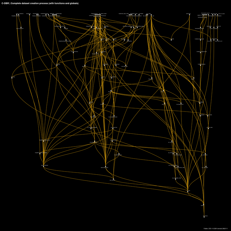
Complete Pipeline (Data, Functions and Globals) Link to heading

A visual of the complete pipeline can be quite intimidating. It displays a harsh beauty, but there is usually too much going on to make much sense of it. Even dynamic tools like the function tar_visnetwork() have trouble making sense of it all. I would recommend exporting the graph to a .graphml file and loading it into Gephi, which is a more convenient tool to view graph diagrams at this level of complexity.

Nonetheless, adding functions and globals to the diagram can provide us with some important clues:

1. Are all functions hooked up to the right targets?
2. Are there dangling functions that are not used in the pipeline?

As you can see, there is a dangling set of three function nodes on the right of this diagram. These are part of an older PDF to TXT extraction workflow that I will probably clean up at a future point in time, but are still part of the project in case I want to refer to them.

Reproducing Data Workflow Diagram Link to heading

To reproduce the above diagram, run the C-DBR pipeline at least once (the pipeline is stored in .Rmd and needs to be rendered to .R first), then execute the below code in the same working directory as the project. You can quickly get the project by git cloning https://github.com/SeanFobbe/c-dbr

The dimensions for the static image are 20x20 inches at 150 dpi as PNG.

Note that every publication of the C-DBR corpus alwys contains a static snapshot visual of the pipeline as PDF/PNG in the analysis archive.

 1library(targets)
 2library(data.table)
 3library(igraph)
 4library(ggraph)
 5
 6edgelist <- tar_network(targets_only = TRUE)$edges
 7setDT(edgelist)
 8
 9g  <- igraph::graph.data.frame(edgelist,
10                               directed = TRUE)
11
12
13ggraph(g,
14       'sugiyama') + 
15    geom_edge_diagonal(colour = "darkgoldenrod2")+
16    geom_node_point(size = 2,
17                    color = "white")+
18    geom_node_text(aes(label = name),
19                   color = "white",
20                   size = 2,
21                   repel = TRUE)+
22    theme_void()+
23    labs(
24        title = paste("C-DBR",
25                      "| Complete dataset creation process (data only)"),
26        caption = "Fobbe | DOI: 10.5281/zenodo.3832111"
27    )+
28    theme(
29        plot.title = element_text(size = 14,
30                                  face = "bold",
31                                  color = "white"),                        
32        plot.background = element_rect(fill = "black"),
33        plot.caption = element_text(color = "white"),
34        plot.margin = margin(10, 20, 10, 10)
35    )

Reproduce Complete Pipeline Diagram (Data, Functions and Globals) Link to heading

The complete pipeline diagram is almost the same as the data workflow above, except that we set tar_network(targets_only = FALSE) and the plot title is slightly different.

To reproduce the above diagram, run the C-DBR pipeline at least once (the pipeline is stored in .Rmd and needs to be rendered to .R first), then execute the below code in the same working directory as the project. You can quickly get the project by git cloning https://github.com/SeanFobbe/c-dbr

The dimensions for the static image are 20x20 inches at 150 dpi as PNG.

Note that every publication of the C-DBR corpus alwys contains a static snapshot visual of the pipeline as PDF/PNG in the analysis archive.

 1library(targets)
 2library(data.table)
 3library(igraph)
 4library(ggraph)
 5
 6
 7edgelist <- tar_network(targets_only = FALSE)$edges
 8setDT(edgelist)
 9
10g  <- igraph::graph.data.frame(edgelist,
11                               directed = TRUE)
12
13ggraph(g,
14       'sugiyama') + 
15    geom_edge_diagonal(colour = "darkgoldenrod2")+
16    geom_node_point(size = 2,
17                    color = "white")+
18    geom_node_text(aes(label = name),
19                   color = "white",
20                   size = 2,
21                   repel = TRUE)+
22    theme_void()+
23    labs(
24        title = paste("C-DBR",
25                      "| Complete dataset creation process (with functions and globals)"),
26        caption = "Fobbe | DOI: 10.5281/zenodo.3832111"
27    )+
28    theme(
29        plot.title = element_text(size = 14,
30                                  face = "bold",
31                                  color = "white"),                        
32        plot.background = element_rect(fill = "black"),
33        plot.caption = element_text(color = "white"),
34        plot.margin = margin(10, 20, 10, 10)
35    )

A Word of Thanks Link to heading

My special thanks go to William Michael Landau and the {targets} contributors for creating such an amazing piece of software. Next to {data.table} and {future} this is one of my all-time favorites of the R ecosystem.