Overview Link to heading

Switching the rows of a matrix by multiplying the matrix with a compatible permutation matrix is an elementary operation in linear algebra. This computational essay shows that interpreting a permutation matrix as a transposed graph and plotting it provides a visual understanding of what the permutation matrix will do.

Visualization may aid in understanding the purpose of permutation matrices, show an interesting link between linear algebra and graph theory, as well as provide an introduction to working with matrices in R.

I assume this post will be primarily of interest to beginners in linear algebra or graph theory, but I originally wrote it to explore permutation matrices for myself.

Permutation Matrices Link to heading

One of the elementary operations in linear algebra is the switching of rows in a matrix. This is particularly useful when solving systems of linear equations through Gaussian Elimination based on the classic $ LU $ factorization.¹

Let us assume we wish to solve the following system of linear equations:

$$ \begin{align} 2y + 3z &= 2 \\ 3x + 5y + 6z &= 1\\ 9z &= 3 \\ \end{align} $$

We can then construct a square matrix $ A_1 $ to represent the coefficients of the left-hand side of this system of equations:

$$ A_1 = \begin{bmatrix} 0 & 2 & 3 \\ 3 & 5 & 6 \\ 0 & 0 & 9 \\ \end{bmatrix} $$

In the course of an $ LU $ factorization we need to find an upper-triangular matrix $ U_1 $ with non-zero pivots (the numbers on the diagonal) and all zeros below the diagonal.² Therefore, in an upper-triangular matrix $ U_1 $ the value in the diagonal at position $ (1,1) $ cannot be zero as it is at the moment.

To achieve this we will want to switch the first and second rows to give the first row a non-zero pivot and save us the bother of performing further row operations on the second row. We can accomplish the switching of the first two rows with the following permutation matrix $ P_1 $:

$$ P_1 = \begin{bmatrix} 0 & 1 & 0 \\ 1 & 0 & 0 \\ 0 & 0 & 1 \\ \end{bmatrix} $$

Our permutation matrix $ P_1 $ does the following:

• A value $ 1 $ in position $ (2,1) $ when multiplied with another matrix $ A_1 $ moves row 1 of $ A_1 $ to row 2.
• Correspondingly, a value $ 1 $ in position $ (1,2) $ when multiplied with another matrix $ A_1 $ moves row 2 of $ A_1 $ to row 1.
• The value $ 1 $ in position $ (3,3) $ means that row 3 stays where it is

In a nutshell: our matrix $ P_1 $ switches rows 1 and 2 with each other and row 3 remains where it is. When we multiply matrix $ P_1 $ with matrix $ A_1 $ we obtain:

$$ P_1A_1 = \begin{bmatrix} 0 & 1 & 0 \\ 1 & 0 & 0 \\ 0 & 0 & 1 \\ \end{bmatrix} \begin{bmatrix} 0 & 2 & 3 \\ 3 & 5 & 6 \\ 0 & 0 & 9 \\ \end{bmatrix} = \begin{bmatrix} 3 & 5 & 6 \\ 0 & 2 & 3 \\ 0 & 0 & 9 \\ \end{bmatrix} = U_1 $$

In terms of the original system of linear equations we would now be solving this form, which presents a more obvious path to a solution:

$$ \begin{align} 3x + 5y + 6z &= 1\\ 2y + 3z &= 2 \\ 9z &= 3 \\ \end{align} $$

With the back substitution algorithm we first solve the last row and obtain $ z = \frac{1}{3} $. We insert $ z $ into the second row and find that $ y = \frac{1}{2} $. Inserting $ y $ and $ z $ into the first row we conclude with $ x = -\frac{7}{6} $.

Note that this is simple example to explain a particular technique and as humans we could have solved the original system of linear equations directly without switching any rows. In cases that include other types of row operations this would not have been possible.

Load Igraph Link to heading

Now to visualize the permutation matrix. For analyzing and visualizing graphs we will rely on {igraph} , one the most comprehensive network analysis packages available in R. While I usually use {ggraph} to visualize graphs, in this simple example {igraph} will do just fine.

1library(igraph)

1## 
2## Attaching package: 'igraph'

1## The following objects are masked from 'package:stats':
2## 
3##     decompose, spectrum

1## The following object is masked from 'package:base':
2## 
3##     union

Input Permutation Matrix $ P_1 $ Link to heading

First we input the permutation matrix into R. By arranging the code a little we can code the matrix almost as we see it.

Nevertheless, it is a good idea to print the stored matrix to make sure the input code is correct. Hard-coding matrices can easily go wrong when columns and rows are switched accidentally. Or when we set nrow or byrow incorrectly.

1P1  <- matrix(c(0, 1, 0, 
2                1, 0, 0, 
3                0, 0, 1),
4              nrow = 3,
5              byrow = TRUE)
6
7print(P1)

1##      [,1] [,2] [,3]
2## [1,]    0    1    0
3## [2,]    1    0    0
4## [3,]    0    0    1

Visualize Small Permutation Matrix $ P_1 $ Link to heading

Now that we have the matrix loaded into R, we create a graph from it. This trick works because a graph can be expressed as a square matrix, so a square matrix can again be interpreted as a graph. The technical term in graph theory is adjacency matrix.

Here we treat the permutation matrix as a directed graph (a ‘digraph’) and transform it first into a graph object, then calculate the transpose, then plot it.³

Note that most of the plotting code below is just to align the optics of the plot with the optics of my website, a simple plot(g1t) call would do just fine.

 1set.seed(999)
 2
 3g1 <- graph_from_adjacency_matrix(P1, mode = "directed")
 4g1t <- t(g1) # Transpose
 5
 6par(bg = "#212121")
 7
 8plot(g1t,
 9     vertex.size = 40,
10     vertex.color = "white")

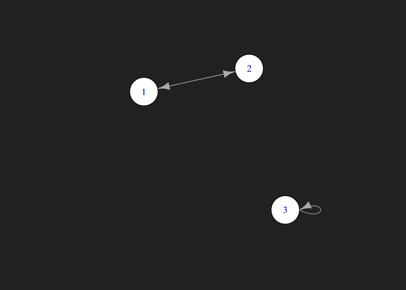
As we expected, the plot shows that rows 1 and 2 are to be switched, while row 3 is left unchanged.

Large Permutation Matrix $ P_2 $ Link to heading

The previous matrix $ P_1 $ was fairly small ( $ n = 3 $ ), but it is interesting to try the exercise with larger matrices, as the advantage of visualization increases with size. The matrices $ P_2 $ and $ A_2 $ are now of size $ n = 5 $ and look a lot more intimidating:

$$ P_2 = \begin{bmatrix} 0 & 0 & 0 & 1 & 0 \\ 0 & 0 & 1 & 0 & 0 \\ 0 & 1 & 0 & 0 & 0 \\ 0 & 0 & 0 & 0 & 1 \\ 1 & 0 & 0 & 0 & 0 \\ \end{bmatrix} \quad A_2 = \begin{bmatrix} 0 & 0 & 0 & 0 & 25\\ 0 & 0 & 13 & 14 & 15\\ 0 & 7 & 8 & 9 & 10\\ 1 & 2 & 3 & 4 & 5\\ 0 & 0 & 0 & 19 & 20\\ \end{bmatrix} $$

Input Large Permutation Matrix $ P_2 $ and Matrix $ A_2 $ Link to heading

We input the two matrices into R and print them to verify that they have been coded correctly:

1P2  <- matrix(c(0, 0, 0, 1, 0, 
2                0, 0, 1, 0, 0, 
3                0, 1, 0, 0, 0, 
4                0, 0, 0, 0, 1, 
5                1, 0, 0, 0, 0),
6              nrow = 5,
7              byrow = TRUE)
8
9print(P2)

1##      [,1] [,2] [,3] [,4] [,5]
2## [1,]    0    0    0    1    0
3## [2,]    0    0    1    0    0
4## [3,]    0    1    0    0    0
5## [4,]    0    0    0    0    1
6## [5,]    1    0    0    0    0

1A2 <- matrix(c(0, 0, 0, 0, 25,
2               0, 0, 13, 14, 15,
3               0, 7, 8, 9, 10,
4               1, 2, 3, 4, 5,
5               0, 0, 0, 19, 20),
6             nrow = 5,
7             byrow = TRUE)
8
9print(A2)

1##      [,1] [,2] [,3] [,4] [,5]
2## [1,]    0    0    0    0   25
3## [2,]    0    0   13   14   15
4## [3,]    0    7    8    9   10
5## [4,]    1    2    3    4    5
6## [5,]    0    0    0   19   20

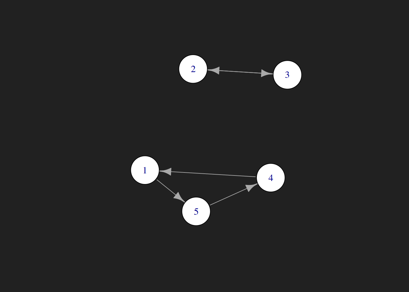
Visualizing the Large Permutation Matrix $ P_2 $ Link to heading

We proceed as we did with the smaller matrix, by creating a graph from an adjacency matrix, then transposing and plotting it. We see that the permutation matrix:

• Rotates rows 1, 4 and 5
• Switches rows 2 and 3 with each other

1g2 <- graph_from_adjacency_matrix(P2, mode = "directed")
2g2t <- t(g2) # Transpose
3
4par(bg = "#212121")
5
6plot(g2t,
7     vertex.size = 40,
8     vertex.color = "white")

Matrix Multiplication Link to heading

To round off this post, let us multiply the matrices $ P_2 $ and $ A_2 $ to make sure that the permutation matrix does exactly what we expect it to do, namely the following:

$$ P_2A_2 = \begin{bmatrix} 0 & 0 & 0 & 1 & 0 \\ 0 & 0 & 1 & 0 & 0 \\ 0 & 1 & 0 & 0 & 0 \\ 0 & 0 & 0 & 0 & 1 \\ 1 & 0 & 0 & 0 & 0 \\ \end{bmatrix} \begin{bmatrix} 0 & 0 & 0 & 0 & 25\\ 0 & 0 & 13 & 14 & 15\\ 0 & 7 & 8 & 9 & 10\\ 1 & 2 & 3 & 4 & 5\\ 0 & 0 & 0 & 19 & 20\\ \end{bmatrix} = \begin{bmatrix} 1 & 2 & 3 & 4 & 5\\ 0 & 7 & 8 & 9 & 10\\ 0 & 0 & 13 & 14 & 15\\ 0 & 0 & 0 & 19 & 20\\ 0 & 0 & 0 & 0 & 25\\ \end{bmatrix} = U_2 $$

We multiply $ P_2 $ with $ A_2 $ in R to obtain:

1U2 <- P2 %*% A2
2print(U2)

1##      [,1] [,2] [,3] [,4] [,5]
2## [1,]    1    2    3    4    5
3## [2,]    0    7    8    9   10
4## [3,]    0    0   13   14   15
5## [4,]    0    0    0   19   20
6## [5,]    0    0    0    0   25

This result matches what we derived from the visualization of the permutation matrix. It worked!

Conclusion Link to heading

It is possible to transform a permutation matrix into a graph, then transpose and plot it to understand what the permutation will do. This may aid in understanding the purpose of permutation matrices, show an interesting link between linear algebra and graph theory, as well as provide an introduction to working with matrices in R.