Overview Link to heading

This tutorial presents the Key Word in Context (KWIC) method, accompanied by code in the R programming language. It guides you through the entire workflow, from first contact with the dataset on Zenodo up to the concluding interpretation and visualization of the results. Additional technical and theoretical background is presented in blue info boxes.

The target audience are lawyers who wish to gain experience with the machine-assisted analysis of texts. We will be analyzing decisions of the International Court of Justice (ICJ). In the course of our analysis the massive amount of text published by the ICJ will be reduced to a human-readable quantity.

KWIC analysis offers the following benefits to lawyers:

• Quick discovery of relevant texts
• Quick discovery of relevant text fragments in relevant texts
• Comprehensive corpus analysis via concordance tables
• Easy visual method to communicate results to non-technical audiences

KWIC analyses are a tried and tested method in natural language processing (NLP). KWIC is all about the discovery of relevant text fragments in a text corpus via keywords or keyphrases. It operates by locating the keyword and extracts a context window (‘in context’) before and after each hit. Lexical dispersion plots offer an attractive and easy to interpret visual representation of KWIC results.

The KWIC method is particularly relevant to the legal domain, because the legal discourse places a premium on highly specific terms to describe legal concepts. Entire court cases may hinge on the interpretation and meaning of particular words. Legal terminology also tend to be archaic and rarely used in everyday writing, which permits the construction of informative queries.

Installation of R Packages Link to heading

This tutorial requires the R packages {zip} , {quanteda} and {quanteda.textplots} . If you haven’t installed them, please do so now.

1install.packages(zip)
2install.packages(quanteda)
3install.packages(quanteda.textplots)

About the Dataset Link to heading

Download and Unpack Dataset Link to heading

 1library(zip)
 2
 3# Download Dataset
 4download.file(url = paste0("https://zenodo.org/records/10030647/files/",
 5                           "CD-ICJ_2023-10-22_EN_CSV_BEST_FULL.zip"),
 6              destfile = "CD-ICJ_2023-10-22_EN_CSV_BEST_FULL.zip")
 7
 8
 9# Unpack Dataset
10unzip(zipfile = "CD-ICJ_2023-10-22_EN_CSV_BEST_FULL.zip")

This part of the code automatically downloads the CSV variant of the ICJ dataset and unpacks it into the local working directory. This does not need to be done with code, a manual download and unzip is fine as well. However, I am relying on code here to show a fully automated and reproducible workflow.

The function paste0() composes the very long URL from two parts: the Zenodo record and the filename. The first reason is aesthetic, because it allows me to break the long line. The second reason is to show you how complex URLs can be constructed programmatically from individual components, a technique that is important in web scraping.

If you do decide to download the dataset manually, please ensure that the file CD-ICJ_2023-10-22_EN_CSV_BEST_FULL.csv is in the same directory as your current working directory. You can check your working directory with getwd(). This is the folder that needs to contain the CSV file.

Reading the Dataset Link to heading

1# Read Dataset from CSV file
2icj <- read.csv(file = "CD-ICJ_2023-10-22_EN_CSV_BEST_FULL.csv",
3                   header = TRUE)
4
5# Select only majority opinions
6icj <- icj[icj$opinion == 0,] 

read.csv() reads the CSV file and assigns it to the object icj. The result is a data.frame, the most commonly used form of table in R. Think of it like an Excel spreadsheet without the gimmicks.

header = TRUE informs the function that the first line of the CSV file contains the names of the variables. Usually this variable is set to TRUE by default, but I wanted to clarify it here for teaching purposes.

For the sake of keeping this tutorial small and runtime short, the second line of code subsets the dataset and limits our analysis to majority opinions only. Omit this line if you also want to look at minority opinions such as declarations, separate opinions and dissenting opinions.

Key Word in Context Analysis (KWIC) Link to heading

Load Quanteda Link to heading

1library(quanteda)

1## Package version: 3.2.1
2## Unicode version: 13.0
3## ICU version: 67.1

1## Parallel computing: 2 of 2 threads used.

1## See https://quanteda.io for tutorials and examples.

1library(quanteda.textplots)

Our KWIC analysis relies on the R package {quanteda} . Quanteda is an excellent and comprehensive framework for natural language processing with extensive documentation.

We will also load {quanteda.textplots} while we are at it. This is an extension to {quanteda} that provides a variety of diagrams to visualize NLP analyses and will come in handy towards the end of the tutorial.

Workflow Link to heading

The diagram shows the NLP workflow we are about to run. It proceeds from the raw data set to creating a corpus object, tokenizing that corpus object, running a KWIC analysis on the tokens and visualizing the result as a lexical dispersion plot.

Usually NLP workflows include some heavy pre-processing, but in the case of KWIC analyses it is better to work with the original texts.

Create Corpus Object Link to heading

1corpus <- corpus(x = icj)

The function corpus() takes a data.frame object and creates a special corpus object that is the basis for the Quanteda NLP workflow. A compatible data.frame must possess the variables doc_id and text to be converted with corpus().

All other variables are interpreted as ‘docvars’, meaning that are understood as metadata attached to the relevant document. The Corpus of Decisions: International Court of Justice (CD-ICJ) is already structured in this format so that you do not have to do anything other than call corpus() on it once.

Tokenization Link to heading

1tokens <- tokens(x = corpus)

Tokenization is a routine step in almost any NLP workflow.

The function tokens() takes a corpus object and outputs a tokens object.

Tokenization breaks down a continuous text (a string, to be precise) into individual parts (tokens). Whitespace is most often used as a token boundary. In Western languages this reflects an intuitive definition of a word but can deviate from intuition when freestanding numbers, special characters or other uncommon sequences of characters are part of the text.¹

For example: the string ‘International Court of Justice’ would be split along whitespace into four tokens: ‘International’, ‘Court’, ‘of’ and ‘Justice’. During tokenization it is common to remove special characters, numbers, emojis and so on. However, we will not remove any content since KWIC works best when the keywords are viewed in their original context.

Run KWIC Analysis Link to heading

1kwic <- kwic(x = tokens,
2             pattern = "terrorism",
3             window = 8,
4             valuetype = "fixed",
5             case_insensitive = TRUE)

The function kwic() runs the Key Word in Context analysis based on a given tokens object.

• x is the primary parameter that defines the tokens input.
• pattern = "terrorism" defines the keyword that is to be searched for.
• window = 8 is the number of tokens before and after the hit to be included in the context window. I’ve set it to 8 tokens, but try different values and observe how the results change.
• value = fixed informs the function that we are looking for a fixed term. Other options are regex or glob to input more complex search expressions.
• case_insensitive = TRUE means that we ignore case during the keyword search. This is often useful because it ignores capitalization errors or can include headings.

The result is a kwic object which we assign the rather obvious but boring name kwic. We will perform a closer analysis soon.

Show Names of Relevant Documents Link to heading

A kwic object is a special type of data.frame. We can therefore use regular data.frame operations to analyze it.

To show all documents with hits we simply select the variable docname and run the function unique() on it to display each name only once.

1unique(kwic$docname)

 1##  [1] "ICJ_070_MilitaryParamilitaryActivitiesNicaragua_NIC_USA_1986-06-27_JUD_01_ME_00_EN.txt"
 2##  [2] "ICJ_088_Lockerbie_LBY_GBR_1992-04-14_ORD_01_NA_00_EN.txt"                              
 3##  [3] "ICJ_088_Lockerbie_LBY_GBR_1998-02-27_JUD_01_PO_00_EN.txt"                              
 4##  [4] "ICJ_089_Lockerbie_LBY_USA_1992-04-14_ORD_01_NA_00_EN.txt"                              
 5##  [5] "ICJ_089_Lockerbie_LBY_USA_1998-02-27_JUD_01_PO_00_EN.txt"                              
 6##  [6] "ICJ_118_ApplicationGenocideConvention_HRV_SRB_2015-02-03_JUD_01_ME_00_EN.txt"          
 7##  [7] "ICJ_121_ArrestWarrant_COD_BEL_2000-12-08_ORD_01_NA_00_EN.txt"                          
 8##  [8] "ICJ_121_ArrestWarrant_COD_BEL_2002-02-14_JUD_01_ME_00_EN.txt"                          
 9##  [9] "ICJ_131_ConstructionWallOPT_UNGA_NA_2004-07-09_ADV_01_NA_00_EN.txt"                    
10## [10] "ICJ_140_ICERD_GEO_RUS_2011-04-01_JUD_01_PO_00_EN.txt"                                  
11## [11] "ICJ_143_JurisdictionalImmunities2008_DEU_ITA_2012-02-03_JUD_01_ME_00_EN.txt"           
12## [12] "ICJ_161_MaritimeDelimitation-IndianOcean_SOM_KEN_2021-10-12_JUD_01_ME_00_EN.txt"       
13## [13] "ICJ_164_IranianAssets_IRN_USA_2019-02-13_JUD_01_PO_00_EN.txt"                          
14## [14] "ICJ_164_IranianAssets_IRN_USA_2023-03-30_JUD_01_ME_00_EN.txt"                          
15## [15] "ICJ_166_ConventionTerrorismFinancingCERD_UKR_RUS_2017-04-19_ORD_01_NA_00_EN.txt"       
16## [16] "ICJ_166_ConventionTerrorismFinancingCERD_UKR_RUS_2017-05-12_ORD_01_NA_00_EN.txt"       
17## [17] "ICJ_166_ConventionTerrorismFinancingCERD_UKR_RUS_2018-09-17_ORD_01_NA_00_EN.txt"       
18## [18] "ICJ_166_ConventionTerrorismFinancingCERD_UKR_RUS_2019-11-08_JUD_01_PO_00_EN.txt"       
19## [19] "ICJ_166_ConventionTerrorismFinancingCERD_UKR_RUS_2019-11-08_ORD_01_NA_00_EN.txt"       
20## [20] "ICJ_166_ConventionTerrorismFinancingCERD_UKR_RUS_2020-07-13_ORD_01_NA_00_EN.txt"       
21## [21] "ICJ_166_ConventionTerrorismFinancingCERD_UKR_RUS_2021-01-20_ORD_01_NA_00_EN.txt"       
22## [22] "ICJ_166_ConventionTerrorismFinancingCERD_UKR_RUS_2021-06-28_ORD_01_NA_00_EN.txt"       
23## [23] "ICJ_166_ConventionTerrorismFinancingCERD_UKR_RUS_2021-10-08_ORD_01_NA_00_EN.txt"       
24## [24] "ICJ_166_ConventionTerrorismFinancingCERD_UKR_RUS_2022-04-08_ORD_01_NA_00_EN.txt"       
25## [25] "ICJ_166_ConventionTerrorismFinancingCERD_UKR_RUS_2022-12-15_ORD_01_NA_00_EN.txt"       
26## [26] "ICJ_166_ConventionTerrorismFinancingCERD_UKR_RUS_2023-02-03_ORD_01_NA_00_EN.txt"       
27## [27] "ICJ_168_Jadhav_IND_PAK_2017-05-18_ORD_01_NA_00_EN.txt"                                 
28## [28] "ICJ_168_Jadhav_IND_PAK_2019-07-17_JUD_01_ME_00_EN.txt"                                 
29## [29] "ICJ_172_ApplicationCERD_QAT_ARE_2018-07-23_ORD_01_NA_00_EN.txt"                        
30## [30] "ICJ_172_ApplicationCERD_QAT_ARE_2021-02-04_JUD_01_PO_00_EN.txt"                        
31## [31] "ICJ_175_1955AmityTreaty_IRN_USA_2018-10-03_ORD_01_NA_00_EN.txt"                        
32## [32] "ICJ_175_1955AmityTreaty_IRN_USA_2021-02-03_JUD_01_PO_00_EN.txt"                        
33## [33] "ICJ_178_ApplicationGenocideConvention_GMB_MMR_2020-01-23_ORD_01_NA_00_EN.txt"          
34## [34] "ICJ_178_ApplicationGenocideConvention_GMB_MMR_2022-07-22_JUD_01_PO_00_EN.txt"          
35## [35] "ICJ_180_ApplicationCERD_ARM_AZE_2021-12-07_ORD_01_NA_00_EN.txt"                        
36## [36] "ICJ_181_ApplicationCERD_AZE_ARM_2021-12-07_ORD_01_NA_00_EN.txt"

Show Number of Hits Link to heading

We can also count the number of hits, that is, how often the keyword was found. With nrow() we obtain the number of rows in the kwic table. This is the same as the number of keyword hits.

1nrow(kwic)

1## [1] 309

Save KWIC Results as a Table Link to heading

That being said, what we really want to look at are the individual hits and their context. The kwic object contains:

• The name of the document
• The position of the hit
• The keyword found (particularly relevant when using wildcards)
• The context window before the hit
• The context window after the hit

To examine the table it is best to export the entire object into a CSV file on disk and inspect it line-by-line with standard spreadsheet software like Excel or Libre Office. For example:

1write.csv(data.frame(kwic), file = "kwic.csv", row.names = FALSE)

Now open the file as you would an ordinary spreadsheet and scroll through it as much as you like.

Inspect KWIC Results in R Link to heading

Since the display of large tables is difficult on the web we will have a look at the first five hits with head():

1head(kwic, n = 5)

 1## Keyword-in-context with 5 matches.                                                                                                
 2##  [ICJ_070_MilitaryParamilitaryActivitiesNicaragua_NIC_USA_1986-06-27_JUD_01_ME_00_EN.txt, 23839]
 3##  [ICJ_070_MilitaryParamilitaryActivitiesNicaragua_NIC_USA_1986-06-27_JUD_01_ME_00_EN.txt, 30640]
 4##  [ICJ_070_MilitaryParamilitaryActivitiesNicaragua_NIC_USA_1986-06-27_JUD_01_ME_00_EN.txt, 30720]
 5##  [ICJ_070_MilitaryParamilitaryActivitiesNicaragua_NIC_USA_1986-06-27_JUD_01_ME_00_EN.txt, 30830]
 6##  [ICJ_070_MilitaryParamilitaryActivitiesNicaragua_NIC_USA_1986-06-27_JUD_01_ME_00_EN.txt, 36657]
 7##                                                            
 8##     prohibit the funds being used for acts of | terrorism |
 9##  , abetting or supporting acts of violence or | terrorism |
10##  , abetting or supporting acts of violence or | terrorism |
11##     Nicaragua was not engaged in support for" | terrorism |
12##  , abetting or supporting acts of violence or | terrorism |
13##                                                
14##  in or against Nicaragua. In June 1984         
15##  in other countries" ( Special Central American
16##  in other countries'". An official             
17##  " abroad, and economic assistance, which      
18##  in other countries, and the press release

Note the long filenames that display information about the case number, title, parties, date type of proceedings and whether it is a majority (“00”) or minority opinion (“01” and higher). This filename is followed by a comma and the position of the hit (only relevant for further machine processing).

Surrounded by the pipe character | in the middle we find our keyword. To the left and right of it, the context window. With this context window we can quickly make the following decisions:

• Which documents are relevant?
• Do the relevant documents contain many hits?
• Are the hits and their context relevant to us? If this is true, then we should closely read the document. If this is not so, then we can quickly remove irrelevant documents from our search.
• Which hits are particularly interesting? In this manner we can quickly discover important fragments of long documents.

Visualization: Lexical Dispersion Plot Link to heading

The presentation in tabular form is important for a detailed analysis. To gain a quick overview of the results visual inspection is best.

Lexical dispersion plots (also called ‘X-ray plot’) are a useful tool to present a KWIC analysis quickly and succinctly. With {quanteda.textplots} and textplot_xray() we can generate such a diagram directly from the kwic object.

The parameter scale = "relative" stipulates that the document length is to be normalized to 1.0. The alternative is scale = "absolute". A relative scale is usually best, since document lengths in legal corpora can vary widely.

1textplot_xray(kwic, scale = "relative")

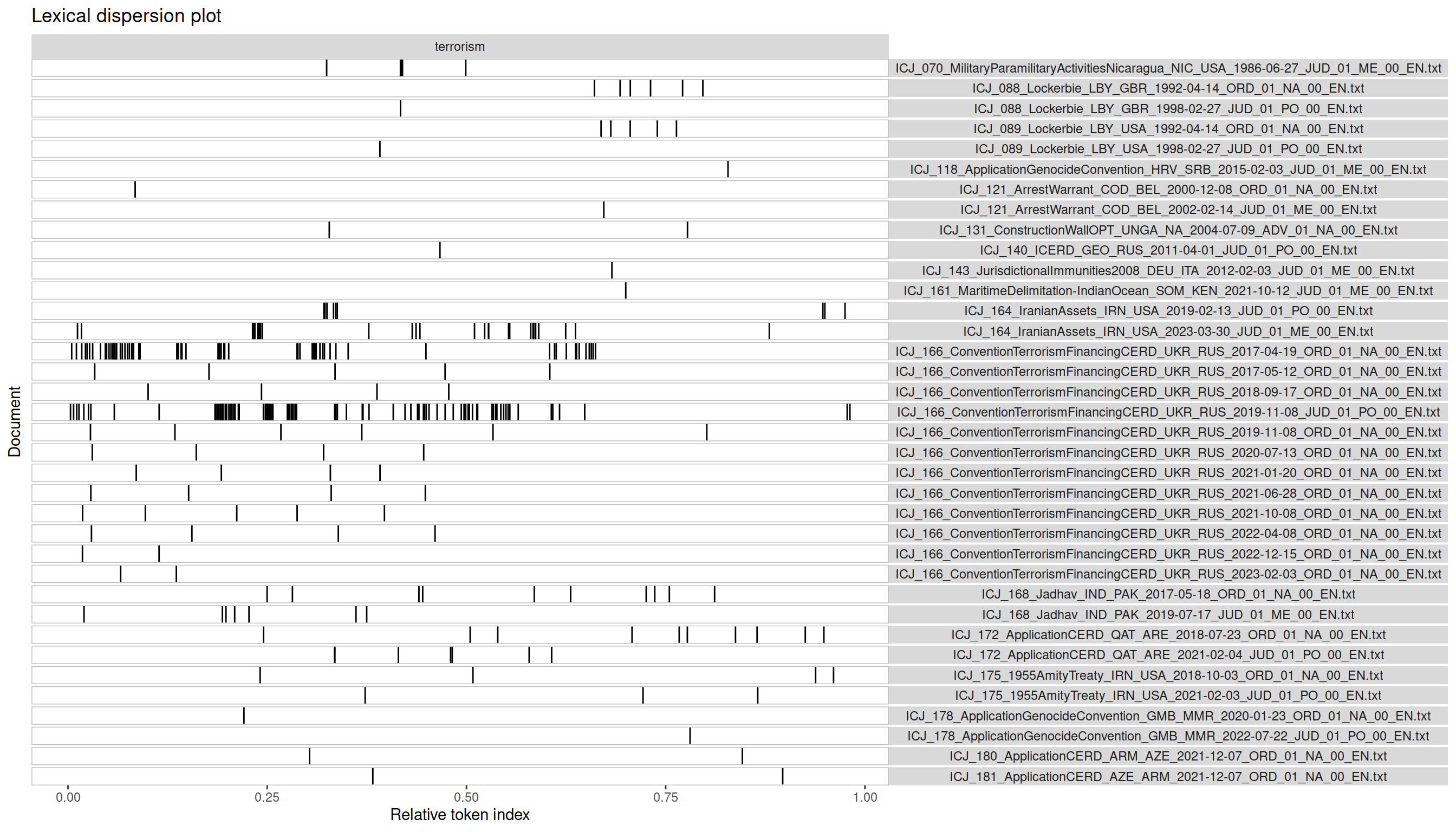
Each row is a document (in this case: an ICJ opinion). The column to the right shows the filename with all the useful metadata mentioned above. The wide column to the left displays hits as black lines. The document length is normalized to 1.0, meaning that a black line at 0.5 is a hit exactly in the middle of the document.

Lexical dispersion plots can help us make some decisions quickly:

• Which documents have many hits and are therefore probably important to our search?
• Which documents have few hits and are therefore probably not important to our search?
• Are there parts of the text in which the keyword is mentioned particularly often, suggesting that we should read them closely?

The diagram clearly shows three opinions as heavily marked by the keyword ’terrorism’: the merits judgment in the Iranian Assets case, the first Order in the Convention on Terrorism Financing and CERD case, as well as the judgment on preliminary objections. All three should be of great interest to any scholar studying the ICJ’s jurisprudence on terrorism.

We also found many more decisions with a few hits. In an academic setting these documents might provide important context or different perspectives on our research question. Practitioners might choose to ignore them entirely. In any case, they can be reviewed quickly with the KWIC CSV table due to the low number of hits.

Conclusion Link to heading

In this tutorial we learned how to apply the Key Word in Context (KWIC) method to a dataset consisting of decisions of the International Court of Justice. We discovered the relevant documents and hits for the keyword ’terrorism’, extracted context windows and gained an overview with a lexical dispersion plot.

A KWIC analysis therefore allows us to:

• Find relevant documents quickly
• Find relevant parts of documents quickly
• Comprehensively analyze an entire corpus
• Create an overview for a non-technical audience (e.g. to discuss results with a client)

Best of luck with applying this method to your own projects!

Replication Details Link to heading

This tutorial was last updated on 2024-02-07.

1sessionInfo()

 1## R version 4.0.4 (2021-02-15)
 2## Platform: x86_64-pc-linux-gnu (64-bit)
 3## Running under: Debian GNU/Linux 11 (bullseye)
 4## 
 5## Matrix products: default
 6## BLAS:   /usr/lib/x86_64-linux-gnu/openblas-pthread/libblas.so.3
 7## LAPACK: /usr/lib/x86_64-linux-gnu/openblas-pthread/libopenblasp-r0.3.13.so
 8## 
 9## locale:
10##  [1] LC_CTYPE=en_US.UTF-8       LC_NUMERIC=C              
11##  [3] LC_TIME=en_US.UTF-8        LC_COLLATE=en_US.UTF-8    
12##  [5] LC_MONETARY=en_US.UTF-8    LC_MESSAGES=en_US.UTF-8   
13##  [7] LC_PAPER=en_US.UTF-8       LC_NAME=C                 
14##  [9] LC_ADDRESS=C               LC_TELEPHONE=C            
15## [11] LC_MEASUREMENT=en_US.UTF-8 LC_IDENTIFICATION=C       
16## 
17## attached base packages:
18## [1] stats     graphics  grDevices utils     datasets  methods   base     
19## 
20## other attached packages:
21## [1] quanteda.textplots_0.94.1 quanteda_3.2.1           
22## 
23## loaded via a namespace (and not attached):
24##  [1] Rcpp_1.0.9         highr_0.9          pillar_1.9.0       bslib_0.4.0       
25##  [5] compiler_4.0.4     jquerylib_0.1.4    tools_4.0.4        stopwords_2.3     
26##  [9] digest_0.6.29      tibble_3.2.1       jsonlite_1.8.0     evaluate_0.15     
27## [13] lifecycle_1.0.3    gtable_0.3.0       lattice_0.20-41    pkgconfig_2.0.3   
28## [17] rlang_1.1.1        Matrix_1.4-1       fastmatch_1.1-3    cli_3.6.1         
29## [21] yaml_2.3.5         blogdown_1.10      xfun_0.31          fastmap_1.1.0     
30## [25] withr_2.5.0        dplyr_1.1.2        stringr_1.5.0      knitr_1.39        
31## [29] generics_0.1.3     vctrs_0.6.2        sass_0.4.2         tidyselect_1.2.0  
32## [33] grid_4.0.4         glue_1.6.2         R6_2.5.1           fansi_1.0.3       
33## [37] rmarkdown_2.14     bookdown_0.27      farver_2.1.1       ggplot2_3.4.2     
34## [41] magrittr_2.0.3     scales_1.2.0       htmltools_0.5.3    colorspace_2.0-3  
35## [45] labeling_0.4.2     utf8_1.2.2         stringi_1.7.8      RcppParallel_5.1.5
36## [49] munsell_0.5.0      cachem_1.0.6